Sequencing Variants Discovery

The Sequencing Variants Toolset Add-In for JMP Pro provides a point-and-click interface to the popular Samtools, Bcftools and HTSlib libraries for the analyses of high-throughput sequencing data.

The goal of the add-in is to provide an easy-to-use interface for calling variants (single nucleotide polymorphisms – SNPs). There are typically many steps of data cleaning and manipulation prior to the variants calling, and the add-in is designed to facilitate the whole process. The add-in include:

•

the ability to index FASTA files

•

the ability to convert SAM to BAM files, and vice-versa,

•

the ability to sort SAM and BAM files (by read name, position, and lexicography),

•

the ability to add mate coordinates to paired-end sequencing reads,

•

the ability to remove duplicated reads

•

the ability to merge BAM (or SAM) files,

•

the ability to index BAM files,

•

the ability to extract subsets of reads (based on criteria such as: mapped, unmapped, properly aligned, from a target region, first read from paired-end sequences),

•

the ability to tag mismatches and insertions,

•

the ability to count reads (by specific flags, by reference, or none),

•

the ability to generate read statistics, base alignment quality statistics, and read depth,

•

the ability to convert VCF to BCF, and vice-versa,

•

the ability to block compress/decompress files (bgzip format), and

•

the ability to generate genotype likelihoods and calls (e.g., SNP calling).

System Requirements

You must have a functional copy of JMP Pro 19 Early Adopter 3 or later. On a Mac, both Intel x86_x64 and Apple Silicon arm64 (M1 and M2) architecture are supported, and should be detected automatically.

Installation

Download the add-in from the JMP Marketplace.

Launch After launching JMP Pro and then open the and click to install.

The installed add-in can be accessed from the JMP Add-Ins menu.

SNP-Calling Workflow

In this section, we will call single nucleotide polymorphisms (SNPs) among three samples of paired-end whole genome sequences of E. coli bacteria.

The Data

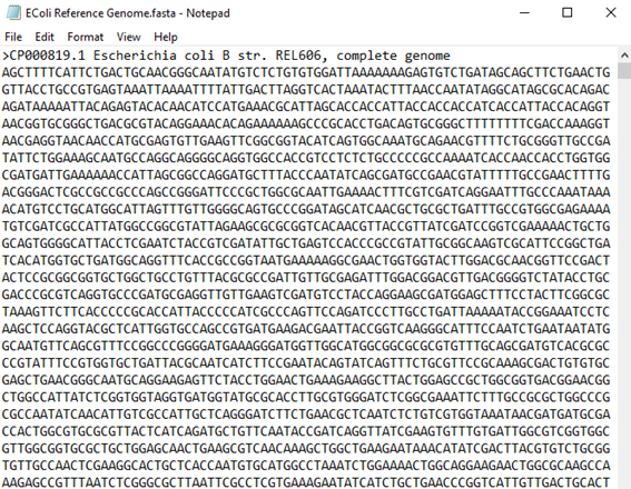
Click Add-Ins > Sequencing Variants Toolset > Example Data > EColi Reference Genome to visualize a reference genome. The content should appear as follows:

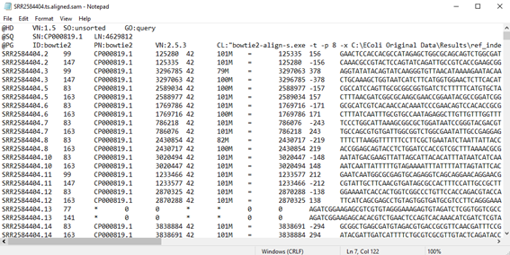
Next, click Add-Ins > Sequencing Variants Toolset > Example Data > SRR2584404 to visualize the sequencing data for sample SRR2584404. The content should appear as follows:

You can repeat the step above to visualize the sequencing data from the other two samples, SRR2584534 and SRR2584666.

The sequences have already been aligned (mapped) to the reference genome with Bowite2 (Langmead and Salzberg, 2012).

The sequencing files are available on a subfolder named Data located under the folder where the add-in got installed. To find out where the add-in was installed in your computer, click View > Add-Ins…, then select Sequencing Variants Toolset.

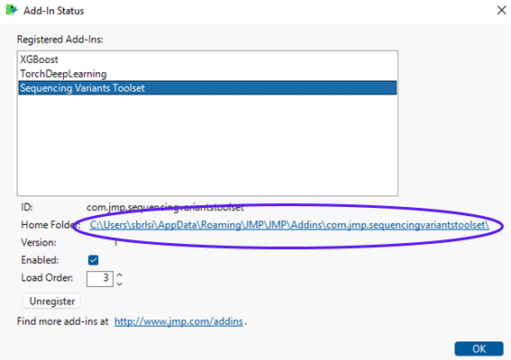
The Home Folder field, circled in the figure above, shows the location where the add-in is installed.

SNP Calls

To call SNPs, click Add-Ins > Sequencing Variants Toolset > Sequencing Variants Toolset to open the add-in interface shown below:

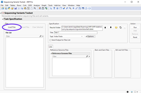
Notice that all fields are blank, except for Results Folder. A good practice when using Samtools and Bcftools libraries is to put input files and output index files all in the same folder. The reason is that some commands in these libraries have pre-defined routines to look for index files in the folder where input files are located. For the sake of simplicity, let’s set the results folder to the current location where input files are installed. If you do not want to write results where the add-in is installed, you could move the input files to another location and set the results folder be that location.

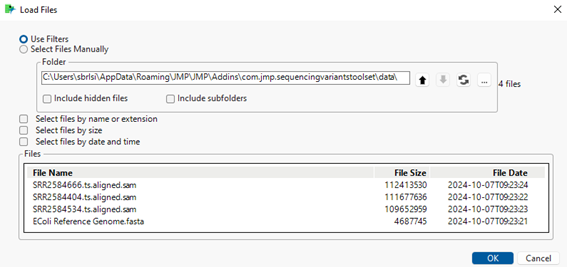
Click (circled below) and navigate to the Data subfolder under the folder where the add-in is installed.

The content should appear as follows:

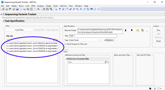
Click to load the files into the Sequencing Variants Toolset interface. The selected files now appear in the File List below.

The following example shows a pipeline to call SNPs from among three sequencing samples.

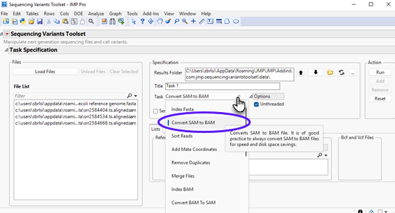
1. Convert SAM files to Bam files.

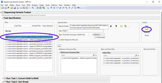
Select Convert SAM to BAM using the Task drop-down menu, as shown below:

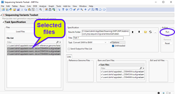
Select the input SAM files on the left panel and click to send selected files to the appropriate field on the right panel. You can select multiple SAM files by clicking on each file and while holding the Ctrl key down. The content should appear as follows:

Click to execute the task. Once it has finished running, you will notice a new report at the bottom window entitled Run: Task 1, Convert SAM to BAM (shown below).

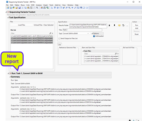
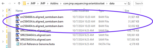
The report shows the command that was executed along with files that were generated. Looking at the results folder, we can see the output BAM files (circled below).

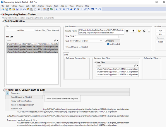
These files will serve as the input files in the next step. To make them available for further analysis, we need to load them into the File List panel.

Click the red triangle located to the left of the report’s title to surface options, then click Send Output to Files List (shown below).

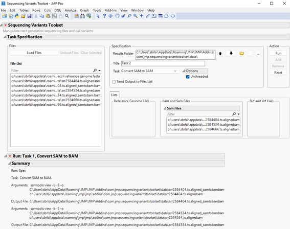
All output BAM files generated in this step will appear in the list of files in the File List panel (shown below).

Before proceeding to the next step, let’s clear all files assigned to the left panels. We can either select all SAM files listed under Sam Files and then click , or click .

2. Sort Reads

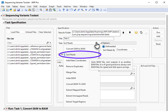
Select Sort Reads using the Task drop-down menu.

Choose Coordinates from the Sort Reads By drop down menu under the Options pane, as shown below.

Select the output BAM files generated in the previous step (listed on the left panel) and click to send them to appropriate panel on the right. Select multiple files by clicking on each file while holding the Ctrl keyboard down. Alternatively, type “.bam” (without double quotes) in the filter field to display only the BAM files in the Files List panel, and then click on a file and hold down Ctrl + A on the keyboard.

The content should appear as follows:

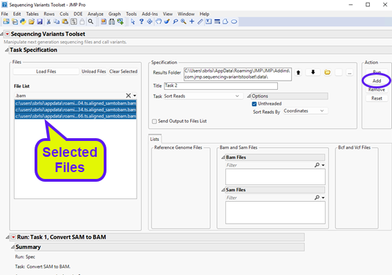
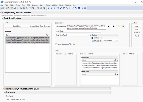
Click to send selected files to the Bam Files panel on the right (see below).

Click to execute the task.

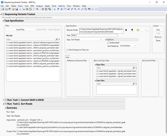
Once it has finished running, you will notice a new report at the bottom window entitled Run: Task 2, Sort Reads (shown below).

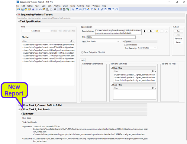
The report shows the command that was executed along with files that were generated. Looking at the results folder, we can see the output sorted BAM files (circled below).

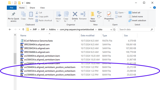
These files will be the input files in the next step. To make them available for further analysis, we need to load them into the File List panel.

Click the red triangle to the left of the report’s title, then click Send Output to Files List (shown below).

Before proceeding to the next step, let’s clear all files assigned to the left panels. We can either select all BAM files listed under Bam Files and then click , or click .

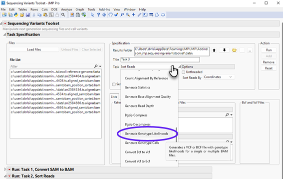
3. Generate Genotype Likelihoods

Select Generate Genotype Likelihoods task in the drop-down, as shown below:

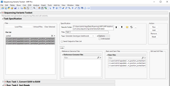
Next, select the output sorted BAM files generated in the previous step (listed on the left panel) and click to send them to the appropriate panel on the right. We can select multiple files by clicking each file and holding the Ctrl keyboard down. Alternatively, you can display only sorted BAM files in the Files List panel by typing “sorted” (without double quotes) in the filter field, and then click on a file and hold down Ctrl + A on the keyboard. The content should appear as follows.

In this step, we need to specify a reference genome file. Select the Ecoli Reference Genome.fasta file in the File List panel and click to send it to the Reference Genome Files panel on the right (show below).

Click to execute the task. Once it has finished running, you will notice a new report at the bottom window entitle Run: Task 3, Generate Genotype Likelihoods (shown below).

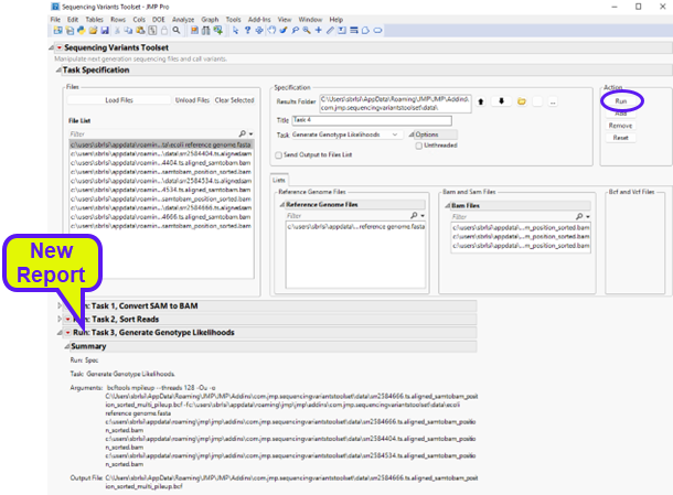
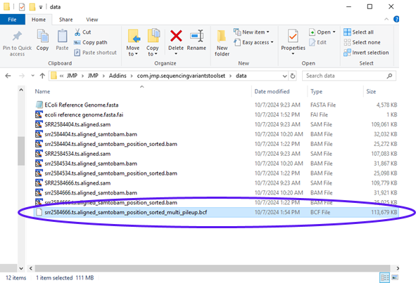
The report shows the command that was executed along with files that were generated. Looking at the results folder, we can see the output BCF file (circled below)..

The output BCF file will be the input file in the next step. To make it available for further analysis, we need to load it into the File List panel.

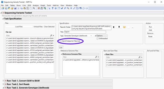
Click the red triangle to the left of the report’s title, then click Send Output to Files List (shown below).

Before proceeding to the next step, you should clear all files assigned to the left panels. We can either select all BAM files listed under Bam Files as well as the reference genome file listed under Reference Genome Files and then click , or click .

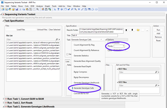
4. Generate Genotype Calls

Select Generate Genotype Calls task in the drop-down menu, and under the Options panel, choose 1 for Ploidy and Multiallelic for Caller from the drop-down menu, as shown below.

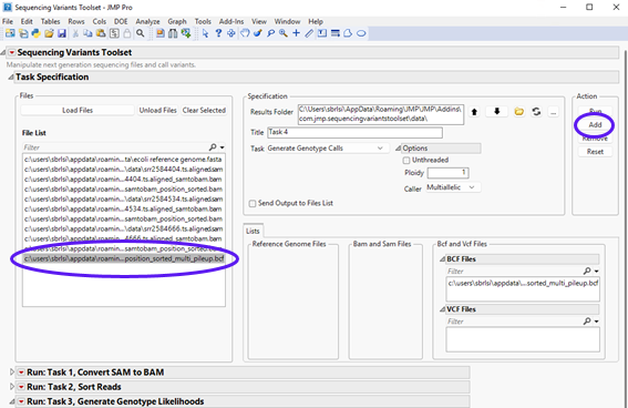
Next, select the output BCF file generated in the previous step (listed on the left panel) and click to send it to the appropriate panel on the right. The content should appear as follows.

Click to execute the task. Once it has finished running, you will notice a new report at the bottom window entitled Run: Task 4, Generate Genotype Calls (shown below).

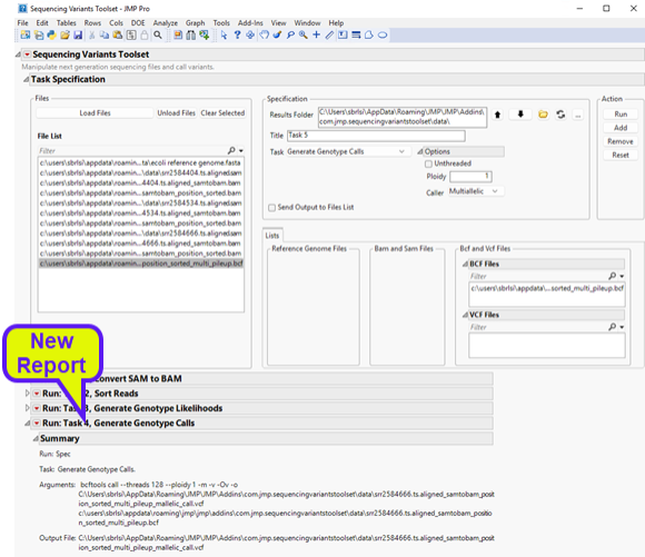
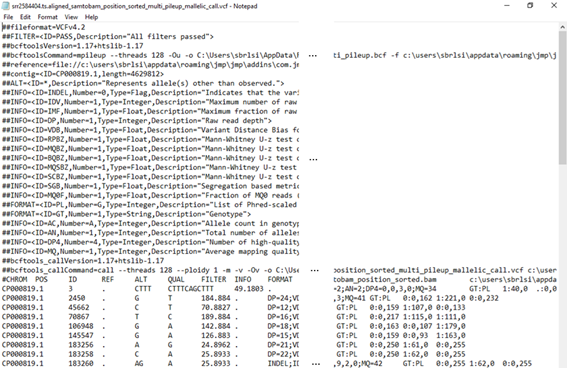
The report shows the command that was executed along with files that were generated. Looking at the results folder, we can see the output VCF file, (circled below).

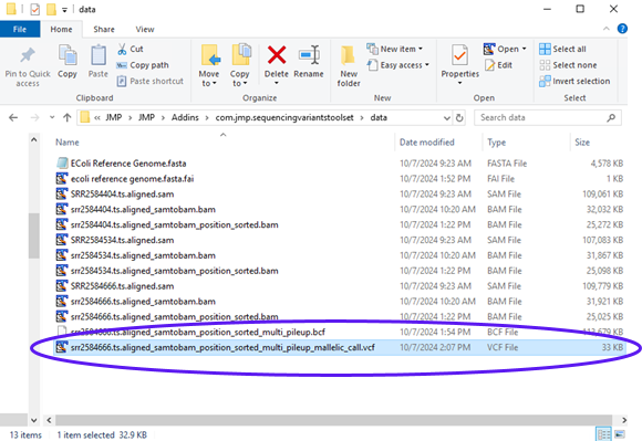
The output VCF file is the final product for this SNP calling example. Its partial content can be seen below.

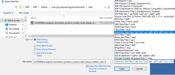
Click File > Open… to open the VCF file (see below).

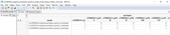
A wide data table with SNPs on the columns and samples on rows is generated. The content should appear as follows

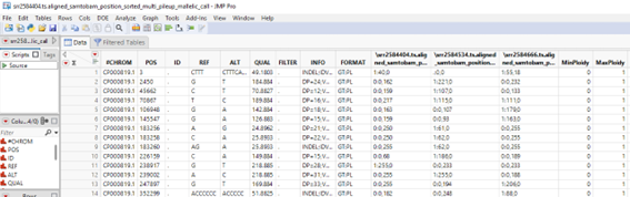
A tall data table with SNPs on the rows and samples on the columns is generated. The content should appear as follows.

References

Langmead B, Salzberg S. 2012. Fast gapped-read alignment with Bowtie 2. Nature Methods 9:357-359.

Danecek P, Bonfield J K, Liddle J, Marshall J, Ohan V, Pollard M O, Whitwham A, Keane T, McCarthy S A, Davies R M, Li H. 2021. Twelve years of SAMtools and BCFtools. GigaScience, Volume 10, Issue 2.